Spatial Analysis
Contents
1. Spatial Analysis#
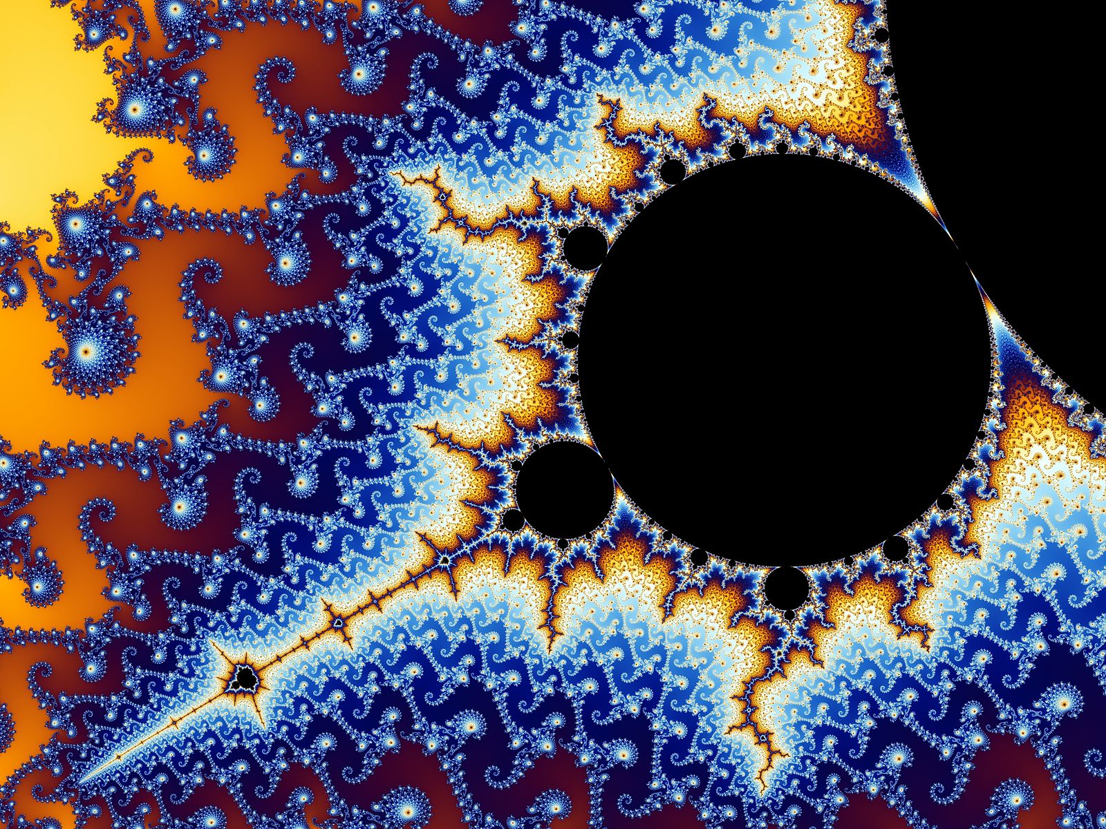
1.1. Fractals#
Coined by Mandelbrot English mathematician
From Latin word “fractus” meaning broken or shattered glass
Refers to irregular objects that are self-similar remaining equally “rough” (or variable) at all scales
Used by Mandelbrot to develop a “theory of roughness”
Fractal Dimensions#
The fractal dimensions (D) describes how an object’s size (S) changes with Linear Scaling (L):
$\(S = L^D\)$
For a simple Euclidean shape the fractal number is an integer: For rectangles and integers, D is 1 is using perimeter to describe size, and 2 if using area to describe size.
For complex shapes (like the coastline of England) the fractal number is a greater number.
Good source on estimating fractal number from data: Davis - Statistical and Data Analysis in Geology
slope = \(\beta\)
Ruler Method:
\(D = 1+\beta\)
Spectral method:
\(D = \frac{5-\beta}{2}\)
1.2. Gridding data#
Form a regular grid: \(\vec{x} (x_i,y_i)\) (for a 2D array of mapped values)
Irregular spaced samples (data): \(\vec{x_k} (x_k,y_k)\) (for 1D array, or list, of sample values)
Goal: Estimate grid vaues \(z_i\) based on the values of the samples (each weighted differently)
How do we weight the data?
Nearest Neighbor#
Use the value of the closest value and ignore all else
Inverse Distance#
Block Average#
Break data up into squares and take the average of each box
1.3. Objective Mapping, Optimal Interpolation, and Krigging#
Interpolation of regular (evenly spaced) grid in two dimensions
Contouring irregularly-spaced data in Python (or Matlab, etc) requires gridding to evenly-spaced points
Best methods: optimal interpolation (aka objective mapping, aka Krigging)
Semivariogram#
\(\vec{x_k}\): measurement locations
\(Z(\vec{x_k})\) = sample values
\(Z(\vec{x_k} + d)\) = sample values at a distance d away from \(\vec{x_k}\)
N(d) = # of measurements that are a distance d away from sample location
Autocovariance#
\(C(d) =\frac{1}{N(d)} \sum^{N(d)}_k [z(\vec{x_k})-\bar{z}(\vec{x})][z(\vec{z_k +d})-\bar{z}(\vec{x})]\)
\(C(d=0) = \sigma ^2\)
Semivariance#
\(\gamma(d) = \frac{1}{2N(d)}\sum^{N(d)}_{k=1}[\vec{Z}(x_k) - Z(\vec{x_k} +d)]^2\)
\(\gamma(d=0) = 0\)
We have already seen examples of autocovariance in time series analysis (like estimating the decorrelation time scale of the Pacific Decadal Oscillation). The semivariance is based on the same concept, but is the opposite. The semivariance is equal to zero at a loag of zero, and plateaus to the variance as distance increases.
Assumptions:#
variables are spatially homogenous
same \(\mu\), \(\sigma\) for any subset
For spatial data \(d\) has units of distance.
For temperature \(\gamma\) has units of \([c]^2\).
Use in mapping and gridding data#
In kriging, objective mapping and optimal interoplation, a model is fit to the semivariogram.
This model is used to determine weights when gridding the data. This provides “optimal” weights based on the covariance structure of the data, without the implicit assumptions of simpler models like the inverse distance model.
This type of analysis also allows a “mapping error” to be computed.
The mapping error reduces to the unresolved variance at zero lag - this includes the variance at smaller scales than those measured or variation in time that occurs as the samples are being collected.
The mapping error is equal to the variance at large scales. In practice, maps often mask regions of high mapping error to avoid misinterpretation of those values.
1.4. Sources with examples and discussion#
Davis - Statistical and Data Analysis in Geology (on reserve) - Seafloor bathymetry and ancient dune topography examples
Glover, Jenkins and Doney - Modeling Methods in Marine Science (on reserve) - Mapping temperature from ARGO floats