Probability and distributions
Contents
2. Probability and distributions#
2.1. Focus questions#
Goals for student knowledge at the end of the lesson:
Give examples of situations where the following distributions are an appropriate model for observed data:
Poission
Weibull
log-normal
normal
Apply Bayes’ theorem to determine probability in cases where trials are not independent.
How does a “prior probability” differ from a “posterior probability” in applications of Bayes’ theorem?
2.2. Probability Density functions#
Probability Functions
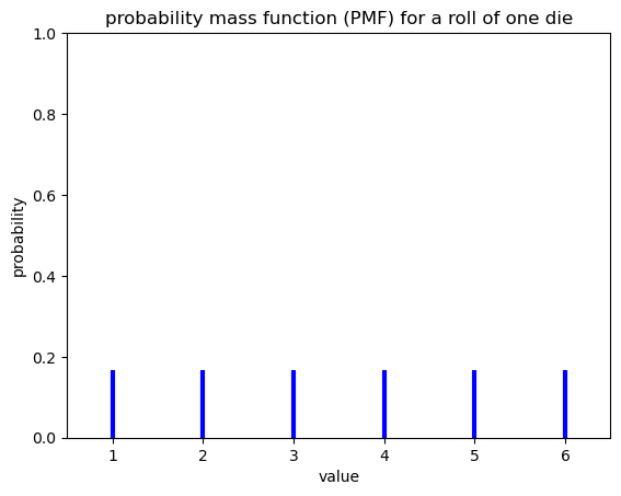
\(P(x)\) = probability mass function (for discrete data)
Example: The probability an number \(x\) coming up on a dice role. The PMF is plotted as vertical lines because the probability of rolling a non-integer (e.g. 3.5) is equal to zero.
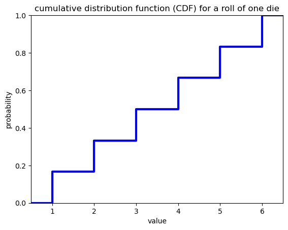
\(F(x)\) = cumulative distribution function (CDF)
The cumulative distribution is the probability of occurrence of a value of \(x\) or lower. For the example of one die roll, the CDF is a step function.
2.3. Formal features of Probabilities#
Mutiplication Principle - If two events \(A\) and \(B\) are unrelated, the probability of joint occurrence \(P(A,B)\), i.e. both events happening, is multiplication of two probabilities,
\(P(A,B) = p(B)p(A)\).
This is a simplification of Bayes’ theorem for the special case where events are independent. In the more general case where the probability of events are not independent,
\(P(A,B) = p(B|A)p(A) = p(A|B)p(B)\),
where \(p(A|B)\) is the probability of \(A\) occuring, given that \(B\) has already occurred. In this case, the two events depend on each other, which is not the case for dice.
Additive principle - Probability of one event or another mutually exclusive event is the sum of the probabilities. Mutually exclusive means that the events cannot occur at the same time.
\(P(C|D) = P(C) + P(D)\)
Bayes theorem – diachronic interpretation#
Diachronic: happening over time
Updating a hypothesis (H) given new data (D):
\(P(H|D) = \frac{P(H)P(D|H)}{P(D)}\)
\(P(H)\) - probability of a hypothesis before seeing data (“prior”)
\(P(H|D)\) - probability of a hypothesis after seeing data (“posterior”)
\(P(D|H)\) - probability of the data given the hypothesis (“likelihood”)
\(P(D)\) - probability of the data under any hypothesis (“normalizing constant”)
\(P(D)\) is often the hardest to understand and quantify
Problems can often be simplified by laying out a suite of hypotheses that are:
Mutually exclusive
Collectively exhaustive
Sum of two dice#
From the rules above, we can calculate the probability mass function and cumulative distribution function for the sum of two dice. From the multiplication rule, the probability of rolling a particular sequence of dice is (1/6) \(\times\) (1/6) = 1/36. This is the probability of a joint occurrence of two independent events. For example, the combinations (1 and 1), (1 and 2), (2 and 1) and (1 and 3) are all joint occurrences of two independent events.
The probability of obtaining a certain sum, which may be arrived at through several possible sequences of dice rolls, can be calculated from the addition rule. There are three ways of obtaining a sum of four: (1 and 3) or (2 and 2) or (3 and 1). These combinations of rolls are mutually exlusive. Therefore the probability of rolling a four is (1/36) + (1/36) + (1/36) = 1/12.
The Monty Hall problem#
A classic application of Bayes theorem, showing how our intuition about probability can lead us astray.
2.4. Distributions#
Normal Distribution#
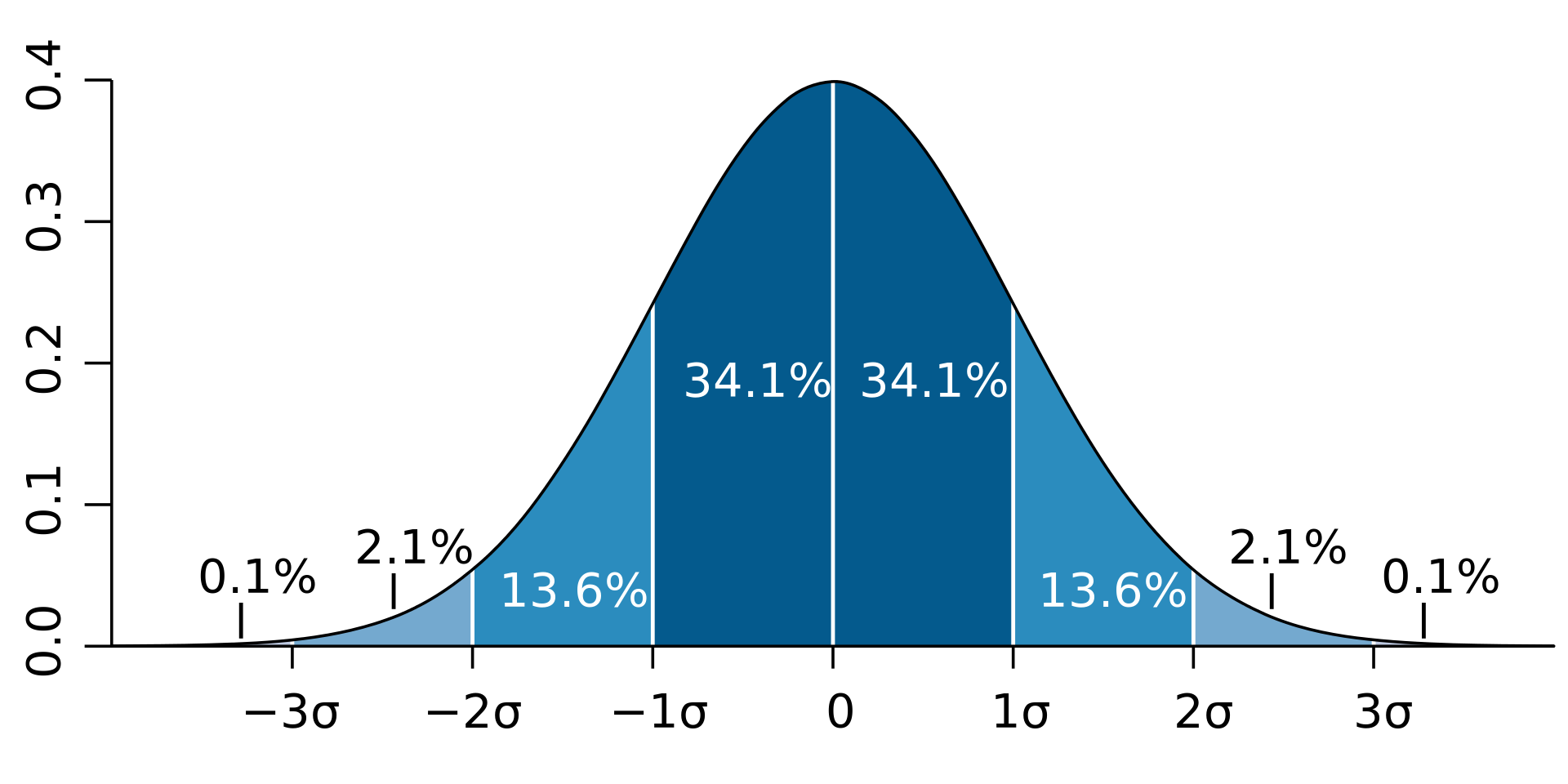
Image credit: Ainali, CC BY-SA 3.0 https://creativecommons.org/licenses/by-sa/3.0, via Wikimedia Commons
Mean - 1st moment
Variance - 2nd moment
Skew - 3rd moment, Describes the spread (Normal Distribution, skew = 0)
Kurtosis - 4th moment, Describes how pointy the distribution is. Low value would be flat (compared to a Normal distribution (k=3))
Non-normal distributions#
Poisson Distribution#
Often used as a model for count data
Assumptions:
One event does not affect the probability of the next (they are independent)
Events cannot occur in the same time and place in the interval
Events occur at a constant rate
\(k\) = # of events counted per interval (ie floods per century)
\(\lambda\) = expected values, true mean
\(P(k) = \frac{\lambda^k e^{-\lambda}}{k!}\)
Count uncertainty = \(\sqrt{k}\) - More counts => less uncertainty
Exercises#
If on average 10 flood occur per century. What is probability of counting 15 floods occuring in a century?
A newspaper article quotes a statistic about the relationship between the El Nino index and high precipitation in Southern California. A high precipitation winter is defined as being in the top 10% of all winters. According to the article, 75% of high precipitation winters in Southern California occur during El Nino years. El Nino events occur approximately every five years. Based on this information, what is the probability of high precipitation occuring during an El Nino year?
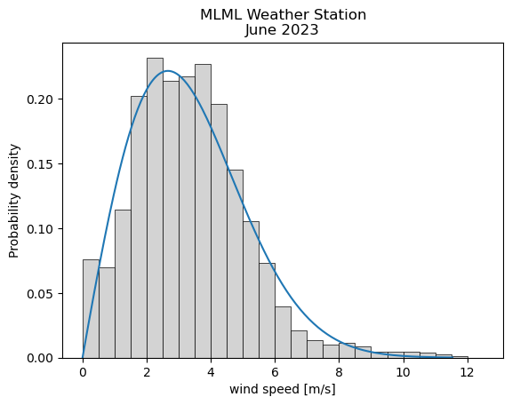
Weibull Distribution#
A theoretical distribution that is often fit to wind speed data. Wind speed has only positive values, so the probability of a negative wind speed is zero. The distribution of wind speed is generally skewed, since very high values do occur, but are rare. This theoretical distribution is useful for engineering wind power projects, since it can be defined by a few parameters. The parameters obtained from a fit to data at a given location can be used as inputs to models for designing equipment with maximum efficiency.
Log-Normal Distribution#
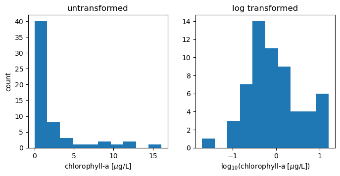
Many biological data, such as growth rates or abundance, follow a log-normal distribution. The distributions are skewed, with a peak close to zero but a long tail of rare high values. These data can be transformed by taking the logarithm, giving a distribution that is more symmetric and closer to a normal distribution.
The example below comes from the distribution of chlorophyll-a samples from the West Coast Ocean Acidification Cruise. Chorophyll-a is a proxy for phyplankton abundance. The untransformed data are highly skewed; low abundaces are common but there are some samples that have very high abundances. Log transforming the data makes the distribution look more “normal,” although it is clearly different from a theoretical Gaussian distribution.
Back to Normal Distributions#
Random instrument error is often normally distributed. The mean of errors tends to be zero if error is randomly distributed and accurate, i.e. not biased.
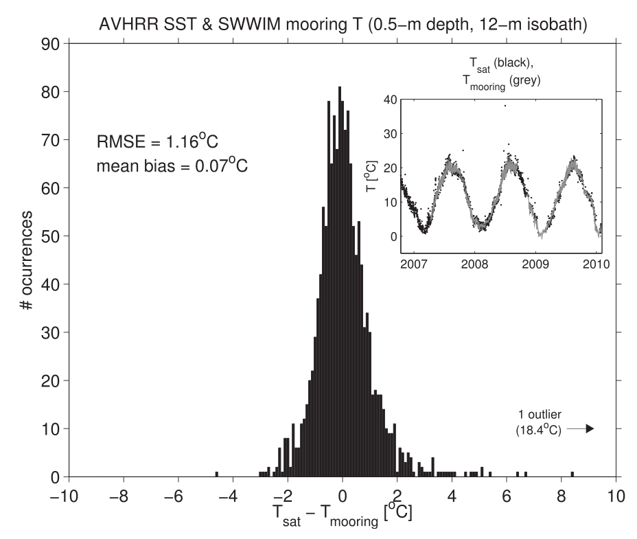
source: Connolly, T. P., & Lentz, S. J. (2014). Interannual variability of wintertime temperature on the inner continental shelf of the Middle Atlantic Bight. Journal of Geophysical Research: Oceans, 119(9), 6269-6285.
In this example, error is defined as: \(T_{sat} - T_{mooring}\) units of [\(^o\)C]. There is a fairly large spread in the data. We therefore cannot be extremely confident in any particular satellite image. However, we can be confident that the mean of a large number of errors is close to zero.
Normal distributions can be “standardized”, where the
mean = 0
standard deviation = 1
Unitless
The z-score transforms the data so that each data point is unitless and described in terms of standard deviations away from the mean.
\(z_i = \frac{x_i - \bar{x}}{ s }\)
The z-score can be helpful for identifying outliers (large Z-scores). Outliers are often classified as having a z-score of \(\pm\) 3. However, the basic rules of scientific integrity require that you have a good reason for excluding outliers from your analysis, and report that they have been excluded. Never delete outliers from the original data set.