8. Poisson regression example

8.1. Modeling tropical storm counts

The number of tropical storms is an example of a variable that is not expected to be normally distributed. Counts cannot be negative, are often skewed and tend to follow a Poisson distribution.

This example follows the general approach of Villarini et al. (2010) in using Poisson regression to model the number of tropical storms based on climate indices.

The goal of Poisson regression is to model a rate of occurrence, \(\Lambda_i\), where the rate changes for each observation \(i\). This model can be expressed as a generalized linear model (GLM) with a logarithmic link function.

\[\log(\Lambda_i) = \beta_0 + \beta_1 x_{1i} + \beta_2 x_{2i} + ... + \beta_n x_{ki}\]

which is the same as

\[\Lambda_i = \exp(\beta_0 + \beta_1 x_{1i} + \beta_2 x_{2i} + ... + \beta_n x_{ki})\]

This is a model for the rate of occurrence \(\Lambda_i\) as a function of \(k\) predictor variables. In this example, the rate of occurrence \(\Lambda_i\) is the number of storm counts per year and each climate index is a predictor variable.

• The logarithmic link function is useful because \(\log(\Lambda_i)\) can be positive or negative, but \(\Lambda_i\) must be positive

• If the data being modeled is a standard Poisson random variable, the model simplifies to \(\Lambda_i = \exp({\beta_0})\)

import numpy as np
import pandas as pd
from matplotlib import pyplot as plt
from scipy import stats
import statsmodels.api as sm
import statsmodels.formula.api as smf

We use a special function to load the climate indices from NOAA.

def read_psl_file(psl_file):
    '''
    Read a data file in in NOAA Physical Sciences Laboratory (PSL) format
    
    Input: String containing the path to a PSL data file
    Returns: Pandas dataframe with monthly data in columns and the year as the index
    
    For a description of the PSL format see: https://psl.noaa.gov/gcos_wgsp/Timeseries/standard/
    '''
    
    f = open(psl_file, "r")
    all_lines = f.readlines()
    start_year = all_lines[0].split()[0]
    end_year = all_lines[0].split()[1]

    for i in range(1,len(all_lines)):
        stri = all_lines[i].find(end_year)
        if stri>=0:
            end_index = i

    missing_val = float(all_lines[end_index+1])
    nrows = int(end_year)-int(start_year)+1
    df = pd.read_csv(psl_file,skiprows=1,nrows=nrows,sep='\s+',header=None,na_values=missing_val)
    df = df.rename(columns={0:'year'})
    df = df.set_index('year',drop=True)
    
    return df

dfsoi = read_psl_file('data/tropical-storms/soi.data')
dftna = read_psl_file('data/tropical-storms/tna.data')
dfnao = read_psl_file('data/tropical-storms/nao.data')

Load the tropical storm data.

dftrop = pd.read_csv('data/tropical-storms/tropical.txt',sep='\t')
dftrop = dftrop.set_index('Year',drop=False)

Tropical storms do not happen in winter, so we average the climate indices during the relevant months.

dftrop['SOI'] = dfsoi.loc[:,5:6].mean(axis=1)
dftrop['TNA'] = dftna.loc[:,5:6].mean(axis=1)
dftrop['NAO'] = dfnao.loc[:,5:6].mean(axis=1)

Exercises

• How would you find the NAO averaged over July-September?

• How would you find the NAO for years 2010-2020, averaged over July-September?

• How would you use dfnao.iloc to achieve the same result?

Drop all rows with any NaN values.

df = dftrop.dropna()

df

	Year	NamedStorms	NamedStormDays	Hurricanes	HurricaneDays	MajorHurricanes	MajorHurricaneDays	AccumulatedCycloneEnergy	SOI	TNA	NAO
Year
1951	1951	12	67.00	8	34.25	3	4.50	126.3	-0.40	0.155	-0.925
1952	1952	11	45.75	5	15.50	2	2.50	69.1	1.20	0.205	-0.545
1953	1953	14	61.75	7	19.00	3	5.00	98.5	-1.30	0.120	0.425
1954	1954	16	57.00	7	26.00	3	7.00	104.4	0.50	0.045	0.015
1955	1955	13	85.50	9	43.00	4	8.50	164.7	1.95	-0.065	-0.530
...	...	...	...	...	...	...	...	...	...	...	...
2016	2016	15	81.00	7	27.75	4	10.25	141.3	0.90	0.385	-0.400
2017	2017	17	93.00	10	51.75	6	19.25	224.9	-0.15	0.590	-0.685
2018	2018	15	87.25	8	26.75	2	5.00	129.0	0.20	-0.440	1.715
2019	2019	18	68.50	6	23.25	3	10.00	129.8	-0.70	0.210	-1.585
2020	2020	30	118.00	13	34.75	6	8.75	179.8	0.05	0.620	-0.085

70 rows × 11 columns

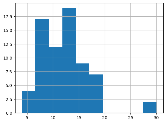
Histogram of the named storm counts.

plt.figure()
df['NamedStorms'].hist()

<Axes: >

Poisson distribution - model as a constant

result = smf.glm(formula='NamedStorms ~ 1',
                 data=df,
                 family=sm.families.Poisson()).fit()
result.summary()

Generalized Linear Model Regression Results

Dep. Variable:	NamedStorms	No. Observations:	70
Model:	GLM	Df Residuals:	69
Model Family:	Poisson	Df Model:	0
Link Function:	Log	Scale:	1.0000
Method:	IRLS	Log-Likelihood:	-206.92
Date:	Tue, 20 Feb 2024	Deviance:	113.91
Time:	18:05:10	Pearson chi2:	123.
No. Iterations:	4	Pseudo R-squ. (CS):	-1.554e-15
Covariance Type:	nonrobust

	coef	std err	z	P>|z|	[0.025	0.975]
Intercept	2.4979	0.034	72.869	0.000	2.431	2.565

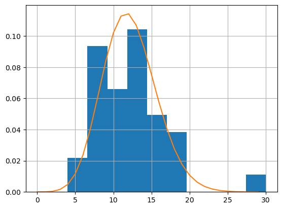
k = np.arange(0,30)
mu = np.exp(result.params.Intercept)
pmf_poisson = stats.poisson.pmf(k,mu)

plt.figure()
df['NamedStorms'].hist(density=True)
plt.plot(k,pmf_poisson)

[<matplotlib.lines.Line2D at 0x15d1ace10>]

Poisson regression model, including a linear temporal trend.

result = smf.glm(formula='NamedStorms ~ Year + NAO + SOI + TNA',
                 data=df,
                 family=sm.families.Poisson()).fit()
result.summary()

Generalized Linear Model Regression Results

Dep. Variable:	NamedStorms	No. Observations:	70
Model:	GLM	Df Residuals:	65
Model Family:	Poisson	Df Model:	4
Link Function:	Log	Scale:	1.0000
Method:	IRLS	Log-Likelihood:	-186.77
Date:	Tue, 20 Feb 2024	Deviance:	73.614
Time:	18:05:10	Pearson chi2:	73.3
No. Iterations:	4	Pseudo R-squ. (CS):	0.4377
Covariance Type:	nonrobust

	coef	std err	z	P>|z|	[0.025	0.975]
Intercept	-8.9786	3.621	-2.480	0.013	-16.076	-1.881
Year	0.0057	0.002	3.154	0.002	0.002	0.009
NAO	-0.0267	0.048	-0.558	0.577	-0.120	0.067
SOI	0.0620	0.037	1.654	0.098	-0.011	0.135
TNA	0.3563	0.096	3.729	0.000	0.169	0.544

beta = result.params

beta

Intercept   -8.978558
Year         0.005747
NAO         -0.026677
SOI          0.061967
TNA          0.356328
dtype: float64

Exercises

• Create a Python variable y that contains the observed count data.

• Create a Python variable yhat that contains the modeled count data (use the parameters in beta).

• Make plots comparing the observed and modeled counts.