Implementing linear regression in Python and matrix review
Contents
5. Implementing linear regression in Python and matrix review#
Like many data analysis problems, there are a number of different ways to perform a linear regression in Python. This notebook shows a few different methods. The final method motivates a review of matrix multiplication, which will be helpful in the next section on multivariate regression.
5.1. Example: 2007 West Coast Ocean Acidification Cruise#
import numpy as np
import pandas as pd
import matplotlib.pyplot as plt

from scipy import stats
import statsmodels.formula.api as smf
import pingouin as pg

import PyCO2SYS as pyco2
5.2. Load data#
Load 2007 data#
filename07 = 'data/wcoa_cruise_2007/32WC20070511.exc.csv'
df07 = pd.read_csv(filename07,header=29,na_values=-999,parse_dates=[[6,7]])
df07.keys()
Index(['DATE_TIME', 'EXPOCODE', 'SECT_ID', 'SAMPNO', 'LINE', 'STNNBR',
       'CASTNO', 'LATITUDE', 'LONGITUDE', 'BOT_DEPTH', 'BTLNBR',
       'BTLNBR_FLAG_W', 'CTDPRS', 'CTDTMP', 'CTDSAL', 'CTDSAL_FLAG_W',
       'SALNTY', 'SALNTY_FLAG_W', 'CTDOXY', 'CTDOXY_FLAG_W', 'OXYGEN',
       'OXYGEN_FLAG_W', 'SILCAT', 'SILCAT_FLAG_W', 'NITRAT', 'NITRAT_FLAG_W',
       'NITRIT', 'NITRIT_FLAG_W', 'PHSPHT', 'PHSPHT_FLAG_W', 'TCARBN',
       'TCARBN_FLAG_W', 'ALKALI', 'ALKALI_FLAG_W'],
      dtype='object')
5.3. Linear regression: five methods in Python#
Create \(x\) and \(y\) variables.
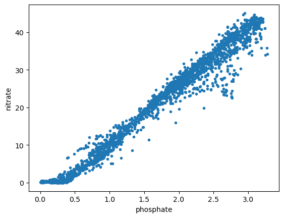
x = df07['PHSPHT']
y = df07['NITRAT']
Plot data.
plt.figure()
plt.plot(x,y,'.')
plt.xlabel('phosphate')
plt.ylabel('nitrate')
Text(0, 0.5, 'nitrate')
Create a subset where both variables have finite values.
ii = np.isfinite(x+y)
ii
0       True
1       True
2       True
3       True
4       True
        ...
2343    True
2344    True
2345    True
2346    True
2347    True
Length: 2348, dtype: bool
Method 1: Scipy#
result = stats.linregress(x[ii],y[ii])
result
LinregressResult(slope=14.740034517902119, intercept=-3.9325720551998167, rvalue=0.9860645445968044, pvalue=0.0, stderr=0.052923783569700955, intercept_stderr=0.10258209230911229)
result.slope
14.740034517902119
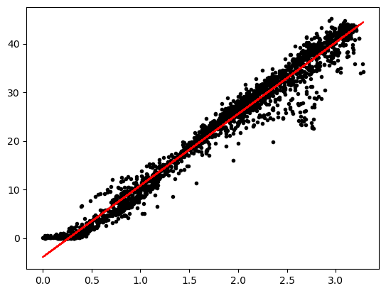
Exercise: Draw the regression line with the data
plt.figure()
plt.plot(x,y,'k.')
plt.plot(x,result.slope*x+result.intercept,'r-')
[<matplotlib.lines.Line2D at 0x152ce6e00>]
/Users/tconnolly/opt/miniconda3/envs/data-book/lib/python3.10/site-packages/outdated/utils.py:14: OutdatedPackageWarning: The package outdated is out of date. Your version is 0.2.1, the latest is 0.2.2.
Set the environment variable OUTDATED_IGNORE=1 to disable these warnings.
  return warn(
Method 2: statsmodels#
Ordinary least squares fit using statsmodels.
smres = smf.ols('NITRAT ~ PHSPHT',df07).fit()
smres.summary()
| Dep. Variable: | NITRAT | R-squared: | 0.972 |
|---|---|---|---|
| Model: | OLS | Adj. R-squared: | 0.972 |
| Method: | Least Squares | F-statistic: | 7.757e+04 |
| Date: | Mon, 13 Jan 2025 | Prob (F-statistic): | 0.00 |
| Time: | 11:28:09 | Log-Likelihood: | -4993.9 |
| No. Observations: | 2210 | AIC: | 9992. |
| Df Residuals: | 2208 | BIC: | 1.000e+04 |
| Df Model: | 1 | ||
| Covariance Type: | nonrobust |
| coef | std err | t | P>|t| | [0.025 | 0.975] | |
|---|---|---|---|---|---|---|
| Intercept | -3.9326 | 0.103 | -38.336 | 0.000 | -4.134 | -3.731 |
| PHSPHT | 14.7400 | 0.053 | 278.514 | 0.000 | 14.636 | 14.844 |
| Omnibus: | 874.728 | Durbin-Watson: | 0.269 |
|---|---|---|---|
| Prob(Omnibus): | 0.000 | Jarque-Bera (JB): | 5147.310 |
| Skew: | -1.766 | Prob(JB): | 0.00 |
| Kurtosis: | 9.589 | Cond. No. | 4.90 |
Notes:
[1] Standard Errors assume that the covariance matrix of the errors is correctly specified.
Method 3: pingouin#
pg.linear_regression(x[ii],y[ii])
/Users/tconnolly/opt/miniconda3/envs/data-book/lib/python3.10/site-packages/outdated/utils.py:14: OutdatedPackageWarning: The package pingouin is out of date. Your version is 0.5.2, the latest is 0.5.5.
Set the environment variable OUTDATED_IGNORE=1 to disable these warnings.
  return warn(
| names | coef | se | T | pval | r2 | adj_r2 | CI[2.5%] | CI[97.5%] | |
|---|---|---|---|---|---|---|---|---|---|
| 0 | Intercept | -3.932572 | 0.102582 | -38.335853 | 6.540950e-247 | 0.972323 | 0.972311 | -4.133740 | -3.731405 |
| 1 | PHSPHT | 14.740035 | 0.052924 | 278.514375 | 0.000000e+00 | 0.972323 | 0.972311 | 14.636249 | 14.843820 |
Method 4: Regression coefficients using numpy’s polyfit function#
We can also use the polyfit function from numpy to calculate the coefficients of the line of best fit (minimizing the sum of square errors):
coefficients = np.polyfit(x[ii],y[ii],1)
print(coefficients)
[14.74003452 -3.93257206]
5.4. Matrix multiplication and linear algebra#
In the next section, we’ll consider solving for the coefficients of the linear fit using matrices. But first, let’s do a quick review of matrix multiplication:
Review: Matrix Multiplication#
Suppose we have the following matrices:
The matrix product \(\textbf{AB}\) is defined by the dot products of the rows of \(\textbf{A}\) and columns of \(\textbf{B}\).
To define matrices in Python, we define 2-d arrays as lists of lists wrapped in numpy’s array function, for example:
# define matrix A
A = np.array([[1, 2, 3],
              [4, 5, 6]])

# define matrix B
B = np.array([[7, 8],
              [9, 10],
              [11, 12]])
We can check the dimensions of these array’s using numpy’s shape function:
print('shape of A: ', np.shape(A))
print('shape of B: ', np.shape(B))
shape of A:  (2, 3)
shape of B:  (3, 2)
Finally, we can multiply two arrays using numpy’s dot function:
np.dot(A,B)
array([[ 58,  64],
       [139, 154]])
Alternatively, we could use np.matmul or the @ operator:
np.matmul(A,B)
array([[ 58,  64],
       [139, 154]])
A@B
array([[ 58,  64],
       [139, 154]])
It is important to remember that matrix multiplication is not commutative, meaning \(\textbf{AB}\) is generally not the same as \(\textbf{BA}\). In this example, \(\textbf{BA}\) gives us a different size matrix.
np.dot(B,A)
array([[ 39,  54,  69],
       [ 49,  68,  87],
       [ 59,  82, 105]])
Review: Matrix Transpose#
The transpose of a matrix \(\textbf{A}^T\) has the same values as \(\textbf{A}\), but the rows are converted to columns. One way to do this is with the np.transpose function.
print(A)
[[1 2 3]
 [4 5 6]]
print(np.transpose(A))
[[1 4]
 [2 5]
 [3 6]]
Another way is to use the .T method on a Numpy array.
print(A.T)
[[1 4]
 [2 5]
 [3 6]]
Note that the product \(\textbf{A}^T\textbf{A}\) is a square matrix, which has the same number of rows and columns.
np.dot(A.T, A)
array([[17, 22, 27],
       [22, 29, 36],
       [27, 36, 45]])
Review: Matrix Inverse#
The concept of a matrix inverse is similar to the matrix of a single number. If we have a single value \(b\), its inverse can be represented as \(b^{-1}\). A value times its inverse is equal to 1.
The inverse of a single number can be used to solve for \(x\) in a linear equation \(bx = c\). For example:
Let’s say we have a square matrix \(\textbf{B}\) where the number of rows and columns are equal. The inverse \(\textbf{B}^{-1}\) is the matrix that gives
where the identity matrix \(\textbf{I}\) is a matrix that has all 0 values, except for 1 values along the diagonal from the upper left to the lower right. For example, a 3x3 identity matrix would be
This is called an identity matrix because \(\textbf{B}\textbf{I} = \textbf{I}\textbf{B} = \textbf{B}\) for square matrices. This is analagous to \(1b = b\) for single values.
In a linear algebra class, you might calculate \(\textbf{B}^{-1}\) by hand, but in this class we will rely in Numpy to do it for us. Let’s set up a \(3 \times 3\) \(\textbf{B}\) matrix.
B = np.array([[1, 2, 1],
              [3, 2, 1],
              [1, 2, 2]])
print(B)
[[1 2 1]
 [3 2 1]
 [1 2 2]]
The inverse \(\textbf{B}^{-1}\) is
np.linalg.inv(B)
array([[-0.5 ,  0.5 ,  0.  ],
       [ 1.25, -0.25, -0.5 ],
       [-1.  ,  0.  ,  1.  ]])
The product \(\textbf{B}^{-1}\textbf{B}\) can be calculated as
BinvB = np.dot(np.linalg.inv(B), B)
print(BinvB)
[[ 1.00000000e+00  3.33066907e-16  1.66533454e-16]
 [-5.55111512e-17  1.00000000e+00 -2.22044605e-16]
 [ 0.00000000e+00  0.00000000e+00  1.00000000e+00]]
If we round these values, we can see more clearly that this is nearly identical to the identity matrix \(\textbf{I}\), with some very small round-off error.
print(np.round(BinvB))
[[ 1.  0.  0.]
 [-0.  1. -0.]
 [ 0.  0.  1.]]
For reference, an identity matrix can be created with the np.eye function
print(np.eye(3))
[[1. 0. 0.]
 [0. 1. 0.]
 [0. 0. 1.]]
Formulating linear regression in matrix form#
We can formulate regression in terms of matrices as
or
Here, \(\vec{\varepsilon}\) represents the vector of errors, or differences between the model and data values.
To solve for the parameters c using matrix multiplication, we first need to fomulate the \(\vec{y}\) and \(\textbf{X}\) matrices
# check to see that the y_subset is only 1-d (and won't work for matrix multiplication)
# print(np.shape(y_subset))

# define an (N, 1 matrix of the y values)
y_matrix = np.reshape(y[ii].ravel(),(len(y[ii]),1))

# print the matrix
print(y_matrix)

# print the shape of the matrix
print('shape of y: ', np.shape(y_matrix))
[[39.14]
 [40.36]
 [42.36]
 ...
 [26.46]
 [25.29]
 [23.98]]
shape of y:  (2210, 1)
# define a matrix X with a column of ones and a column of the x values
X = np.column_stack([np.ones((len(x[ii]),1)),
                     np.ravel(x[ii])])

# print the X matrix
print(X)

# print the shape of the X matrix
print(np.shape(X))
[[1.   2.73]
 [1.   2.83]
 [1.   2.94]
 ...
 [1.   2.35]
 [1.   2.26]
 [1.   2.1 ]]
(2210, 2)
Now that we have our matrices set up, let’s return to our model equation in matrix form.
We can multiply each side of the equation by the transpose
then multiply each side by the inverse of \(\textbf{X}^T\textbf{X}\)
Since which reduces to
giving us an expression for the vector of coefficents \(\vec{c}\).
Here \(\hat{y}\) represents the vector of model values. With the vector of data values \(\vec{y}\) we can solve for the coefficients that minimize the sum of square errors using the same equation:
Using numpy, we can define the matrix components of the above equation and then run the calculation to find the coefficients:
# calculate the transpose of the matrix X
XT = np.transpose(X)

# calculate the product of XT and X
XTX = np.dot(XT,X)

# calculate the inverse of XTX
XTX_inverse = np.linalg.inv(XTX)

# then calculate the products of XTX, XT and using two dot products
c = np.dot(XTX_inverse,np.dot(XT,y_matrix))

# print the coefficients
print(c)
[[-3.93257206]
 [14.74003452]]
As a sanity check, we can double check that the coefficients are the same as those from numpy’s polyfit function
coefficients = np.polyfit(x[ii],y[ii],1)
print(coefficients)
[14.74003452 -3.93257206]