Multidimensional Scaling Analysis
Contents
2. Multidimensional Scaling Analysis#
Multidimensional scaling analysis (MDS) provides a visual representation of similarity between samples that have multiple variables. MDS is built on the idea of a distance matrix that quantifies the dissimilarity between samples.
2.1. Euclidean Distance#
How far away two points are when plotted as \(x\),\(y\) coordinates.
For three variables, the distance between two samples (\(i\) and \(j\)) can be visualized in three-dimensional space.
\(d_{ij} =||X_i-X_j|| = \sqrt{(x_i-x_j)^2 + (y_i-y_j)^2 + (z_i-z_j)^2}\)
if \(X_i = (x_{i}, y_{i}, z_{i})\)
2.2. Bray Curtis Distance#
Often used for identifying differences in community composition based on abundance. If \(u\) and \(v\) represent two different samples of counts of different groups, the Bray Curtis distance is:
\(d= \frac{\Sigma|u_i-v_i|}{\Sigma(u_i+v_i)}\)
if \(u\) and \(v\) are positive, then 0 < d < 1
Example#
In this example, \(u\), \(v\) and \(q\) are three different samples, in which four different groups are counted.
import numpy as np
from scipy.spatial import distance
u = [415,200,310,411]
v = [615,100,330,203]
q = [614,101,331,202]

data = np.array([u,v,q])
print(data)
[[415 200 310 411]
 [615 100 330 203]
 [614 101 331 202]]
data.T # Transpose so that each column represents a sample
array([[415, 615, 614],
       [200, 100, 101],
       [310, 330, 331],
       [411, 203, 202]])
# compute distances between points
dist = distance.pdist(data,'braycurtis')
dist
array([0.20433437, 0.20433437, 0.00160256])
# represent distances as a matrix
distmatrix = distance.squareform(dist)
distmatrix
array([[0.        , 0.20433437, 0.20433437],
       [0.20433437, 0.        , 0.00160256],
       [0.20433437, 0.00160256, 0.        ]])
2.3. Other measures of distance#
Python can be used to compute a variety of different distance measures.
https://docs.scipy.org/doc/scipy/reference/spatial.distance.html
For an excellent resource on the applications of different distance calculations in ecology, including appropriate measures for binary (presence/absence) data, see A Primer of Ecological Statistics by Gotelli and Ellison.
2.4. Types of multidimensional scaling analysis#
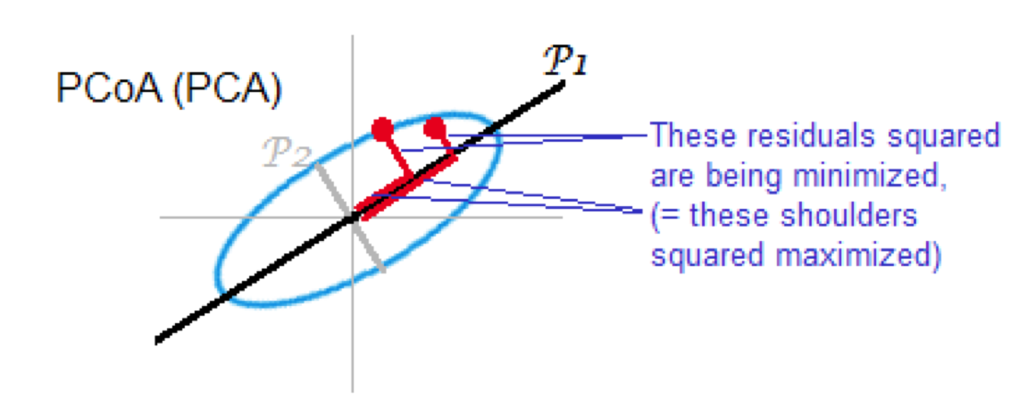
classical MDS
Also known as Torgerson MDS or principal coordinate analysis (PCoA)
The distance matrix is converted to a similarity matrix. Once this is done, the same steps as PCA are performed:
compute eigenvectors and eigenvalues
same as PCA for Euclidean distances
Steps:
create a data matrix
compute a dissimilarity matrix, D, with elements \(d_{ij}\)
transform the dissimilarity matrix \(d^*_{ij} = \frac{1}{2}d^2_{ij}\)
center the dissimilarity matrix \(\delta^*_{ij} = d^*_{ij}-\bar{d}^*_{i}-\bar{d}^*_{j}+\bar{d}^*\)
compute the eigenvectors and eigenvalues
if the dissimilarity index is euclidean distance, this is mathematically equivalent to PCA
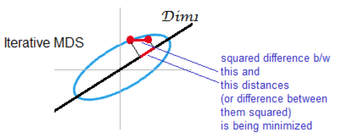
Non-metric (iterative) MDS
preserves rank of distance
minimizes stress
2.5. Summary of comparison of PCA and MDS#
PCA - based on Euclidean distances, good for data without strong skew & data without outliers
PCoA - use when other distance measures are appropriate equivalent to PCA when Euclidean distances used
Non-metric multidimensional scaling (NMDS) - preserves ran order of distance rather than actual values (similar to many non-parametric statistics. One reason for using this type of analysis is that it is less sensitive to outliers.
2.6. ANOSIM and PermANOVA#
determine whether groups of samples are significantly different
are distances WITHIN the groups smaller than the differences BETWEEN groups
2.7. Implementing MDS in Python#
Compute distance matrices
Includes PCA functions
Includes PCoA (metric MDS based on distance matrix)
Does not include non-metric MDS
Includes PermANOVA for assessing statistically significant differences
Computes distance matrices
Includes general MDS function (metric or non-metric)
Includes related analyses such as linear discriminant analysis