Multivariate regression tutorial: aragonite saturation state
Contents
7. Multivariate regression tutorial: aragonite saturation state#
Using data from the West Coast Ocean Acidification (WCOA) cruise, create two different multiple linear regression models to calculate aragonite saturation state (\(\Omega_A\)) between 30 and 300 dbar as a function of more commonly observed variables. This is similar to “Model 1” described in the previous section, following Juranek et al. (2009). Note that there are a couple of issues with this model that led Juranek et al. (2009) to select a different model: bias and multicollinearity.
Juranek, L. W., R. A. Feely, W. T. Peterson, S. R. Alin, B. Hales, K. Lee, C. L. Sabine, and J. Peterson, 2009: A novel method for determination of aragonite saturation state on the continental shelf of central Oregon using multi-parameter relationships with hydrographic data. Geophys. Res. Lett., 36, doi:10.1029/2009GL040778.
First import the necessary packages and load the data.
import numpy as np
import matplotlib.pyplot as plt
import pandas as pd

from scipy import stats
import statsmodels.api as sm
import statsmodels.formula.api as smf
import pingouin as pg

import PyCO2SYS as pyco2
/Users/tconnolly/opt/miniconda3/envs/data-book/lib/python3.10/site-packages/outdated/utils.py:14: OutdatedPackageWarning: The package pingouin is out of date. Your version is 0.5.2, the latest is 0.5.5.
Set the environment variable OUTDATED_IGNORE=1 to disable these warnings.
  return warn(
/Users/tconnolly/opt/miniconda3/envs/data-book/lib/python3.10/site-packages/outdated/utils.py:14: OutdatedPackageWarning: The package outdated is out of date. Your version is 0.2.1, the latest is 0.2.2.
Set the environment variable OUTDATED_IGNORE=1 to disable these warnings.
  return warn(
filename07 = 'data/wcoa_cruise_2007/32WC20070511.exc.csv'
df07 = pd.read_csv(filename07,header=29,na_values=-999,
                  parse_dates=[[6,7]])
We use the PyCO2SYS package to calculate the carbonate system parameters. This gives us values for aragonite saturation state that we can put in our dataframe.
c07 = pyco2.sys(df07['ALKALI'], df07['TCARBN'], 1, 2,
               salinity=df07['CTDSAL'], temperature=df07['CTDTMP'],
                pressure=df07['CTDPRS']);
df07['OmegaA'] = c07['saturation_aragonite'];
/Users/tconnolly/opt/miniconda3/envs/data-book/lib/python3.10/site-packages/autograd/tracer.py:48: RuntimeWarning: invalid value encountered in sqrt
  return f_raw(*args, **kwargs)
/Users/tconnolly/opt/miniconda3/envs/data-book/lib/python3.10/site-packages/PyCO2SYS/equilibria/p1atm.py:99: RuntimeWarning: invalid value encountered in sqrt
  lnKF = 1590.2 / TempK - 12.641 + 1.525 * IonS**0.5
/Users/tconnolly/opt/miniconda3/envs/data-book/lib/python3.10/site-packages/PyCO2SYS/equilibria/p1atm.py:577: RuntimeWarning: overflow encountered in power
  K1 = 10.0 ** -(pK1)
/Users/tconnolly/opt/miniconda3/envs/data-book/lib/python3.10/site-packages/PyCO2SYS/equilibria/p1atm.py:583: RuntimeWarning: overflow encountered in power
  K2 = 10.0 ** -(pK2)
/Users/tconnolly/opt/miniconda3/envs/data-book/lib/python3.10/site-packages/PyCO2SYS/equilibria/p1atm.py:603: RuntimeWarning: overflow encountered in power
  K1 = 10.0**-pK1
/Users/tconnolly/opt/miniconda3/envs/data-book/lib/python3.10/site-packages/PyCO2SYS/equilibria/p1atm.py:611: RuntimeWarning: overflow encountered in power
  K2 = 10.0**-pK2
/Users/tconnolly/opt/miniconda3/envs/data-book/lib/python3.10/site-packages/PyCO2SYS/equilibria/p1atm.py:636: RuntimeWarning: overflow encountered in power
  K1 = 10.0**-pK1
/Users/tconnolly/opt/miniconda3/envs/data-book/lib/python3.10/site-packages/PyCO2SYS/equilibria/p1atm.py:641: RuntimeWarning: overflow encountered in power
  K2 = 10.0**-pK2
/Users/tconnolly/opt/miniconda3/envs/data-book/lib/python3.10/site-packages/PyCO2SYS/equilibria/p1atm.py:653: RuntimeWarning: overflow encountered in power
  K1 = 10.0**-pK1
/Users/tconnolly/opt/miniconda3/envs/data-book/lib/python3.10/site-packages/PyCO2SYS/equilibria/p1atm.py:658: RuntimeWarning: overflow encountered in power
  K2 = 10.0**-pK2
/Users/tconnolly/opt/miniconda3/envs/data-book/lib/python3.10/site-packages/PyCO2SYS/equilibria/p1atm.py:715: RuntimeWarning: overflow encountered in power
  K2 = 10.0**-pK2
/Users/tconnolly/opt/miniconda3/envs/data-book/lib/python3.10/site-packages/PyCO2SYS/solubility.py:41: RuntimeWarning: overflow encountered in power
  KAr = 10.0**logKAr  # this is in (mol/kg-SW)^2
/Users/tconnolly/opt/miniconda3/envs/data-book/lib/python3.10/site-packages/PyCO2SYS/solubility.py:25: RuntimeWarning: overflow encountered in power
  KCa = 10.0**logKCa  # this is in (mol/kg-SW)^2 at zero pressure
7.1. Model 1: Temperature, salinity, pressure, dissolved oxygen and nitrate:#
Temperature
Salinity
Pressure
Oxygen
Nitrate
First, create a subset of all good data between 30-300 dbar.
ii = ((df07['CTDPRS'] >= 30) & (df07['CTDPRS'] <= 300) &
      (df07['NITRAT_FLAG_W'] ==2) & (df07['PHSPHT_FLAG_W'] ==2) &
      (df07['CTDOXY_FLAG_W'] == 2) & (df07['CTDSAL_FLAG_W'] ==2) &
      (df07['TCARBN_FLAG_W'] == 2) & (df07['ALKALI_FLAG_W'] == 2) &
      (df07['LATITUDE'] > 41) & (df07['LATITUDE'] < 48))
df07sub = df07[ii]
y = df07sub['OmegaA']
Solve for the coefficients \(\vec{c}\) in the least squares problem:
Create a 2-D array X that contains a column of all ones, and additional columns containing the explanatory variables. This 2-D array is called the “design matrix” and should have six columns. What are the explanatory variables in this case?
Approach: use
np.ones()to create a 2-D array of correct size, then fill in the columns.
k = 5 # number of predictor variables
N = len(df07sub['OmegaA']) # number of observations
N
159
X = np.ones([N, k+1])
np.shape(X)
(159, 6)
X[:,1] = df07sub['CTDTMP']
X[:,2] = df07sub['CTDSAL']
X[:,3] = df07sub['CTDPRS']
X[:,4] = df07sub['CTDOXY']
X[:,5] = df07sub['NITRAT']
X
array([[  1.   ,   6.395,  33.91 , 250.   , 114.9  ,  31.63 ],
       [  1.   ,   7.163,  33.8  , 175.2  , 145.2  ,  27.63 ],
       [  1.   ,   7.131,  33.65 , 152.2  , 182.3  ,  24.67 ],
       [  1.   ,   7.727,  33.38 , 131.2  , 186.5  ,  23.01 ],
       [  1.   ,   8.203,  32.7  , 109.3  , 259.9  ,  11.88 ],
       [  1.   ,   8.266,  32.47 ,  89.5  , 286.7  ,   7.1  ],
       [  1.   ,   8.624,  32.42 ,  70.5  , 294.7  ,   5.9  ],
       [  1.   ,   8.754,  32.39 ,  60.6  , 297.5  ,   5.61 ],
       [  1.   ,   9.656,  32.39 ,  49.1  , 300.7  ,   4.56 ],
       [  1.   ,  10.23 ,  32.39 ,  38.7  , 298.4  ,   4.1  ],
       [  1.   ,  10.683,  32.39 ,  30.4  , 295.1  ,   3.95 ],
       [  1.   ,   6.877,  33.99 , 249.8  ,  74.6  ,  33.81 ],
       [  1.   ,   7.55 ,  33.9  , 174.5  , 101.9  ,  30.   ],
       [  1.   ,   8.012,  33.74 , 128.9  , 126.6  ,  27.95 ],
       [  1.   ,   7.944,  32.84 ,  89.3  , 234.4  ,  14.97 ],
       [  1.   ,   8.507,  32.49 ,  71.1  , 280.5  ,   7.55 ],
       [  1.   ,   8.709,  32.44 ,  60.3  , 286.5  ,   6.3  ],
       [  1.   ,   8.962,  32.43 ,  49.1  , 294.2  ,   5.69 ],
       [  1.   ,   9.713,  32.43 ,  39.7  , 297.   ,   4.4  ],
       [  1.   ,  10.6  ,  32.46 ,  30.4  , 292.4  ,   3.79 ],
       [  1.   ,   6.863,  33.91 , 174.6  , 108.7  ,  32.75 ],
       [  1.   ,   7.171,  33.87 , 150.   , 115.6  ,  30.78 ],
       [  1.   ,   7.474,  33.79 , 130.7  , 124.1  ,  29.71 ],
       [  1.   ,   7.647,  33.65 , 110.8  , 138.3  ,  28.23 ],
       [  1.   ,   7.656,  33.45 ,  89.8  , 159.   ,  26.62 ],
       [  1.   ,   7.739,  33.01 ,  70.2  , 196.8  ,  21.97 ],
       [  1.   ,   8.035,  32.35 ,  39.6  , 285.3  ,   8.51 ],
       [  1.   ,   8.686,  32.22 ,  30.2  , 291.   ,   5.82 ],
       [  1.   ,   7.717,  33.65 ,  70.3  , 134.7  ,  27.72 ],
       [  1.   ,   7.777,  33.41 ,  60.   , 162.8  ,  24.15 ],
       [  1.   ,   8.005,  33.08 ,  50.2  , 197.8  ,  19.16 ],
       [  1.   ,   8.037,  32.63 ,  39.9  , 233.5  ,  15.76 ],
       [  1.   ,   8.353,  32.29 ,  30.1  , 246.4  ,  11.94 ],
       [  1.   ,   8.047,  33.74 , 109.2  ,  95.3  ,  30.47 ],
       [  1.   ,   8.366,  33.28 ,  90.2  , 162.6  ,  23.74 ],
       [  1.   ,   8.887,  32.52 ,  60.   , 269.1  ,   9.61 ],
       [  1.   ,   9.022,  32.44 ,  50.6  , 284.7  ,   6.68 ],
       [  1.   ,   9.491,  32.39 ,  40.2  , 289.1  ,   5.68 ],
       [  1.   ,  10.132,  32.33 ,  30.8  , 291.4  ,   3.77 ],
       [  1.   ,   5.973,  34.08 , 299.5  ,  43.4  ,  37.99 ],
       [  1.   ,   6.048,  34.07 , 274.3  ,  45.5  ,  37.83 ],
       [  1.   ,   6.078,  34.07 , 250.1  ,  46.3  ,  37.65 ],
       [  1.   ,   6.198,  34.06 , 224.9  ,  50.5  ,  37.35 ],
       [  1.   ,   7.101,  33.99 , 199.8  ,  73.4  ,  34.1  ],
       [  1.   ,   7.471,  33.94 , 174.3  ,  86.6  ,  32.55 ],
       [  1.   ,   7.849,  33.84 , 150.2  , 104.7  ,  30.34 ],
       [  1.   ,   7.945,  33.77 , 130.1  , 117.6  ,  29.1  ],
       [  1.   ,   8.236,  33.63 , 111.8  , 136.9  ,  27.   ],
       [  1.   ,   8.547,  33.01 ,  90.1  , 208.5  ,  19.34 ],
       [  1.   ,   8.723,  32.48 ,  69.7  , 269.3  ,   9.41 ],
       [  1.   ,   8.932,  32.44 ,  60.9  , 283.1  ,   7.24 ],
       [  1.   ,   9.243,  32.4  ,  50.2  , 283.3  ,   6.42 ],
       [  1.   ,   9.891,  32.39 ,  39.6  , 284.   ,   4.94 ],
       [  1.   ,   6.674,  34.03 , 299.6  ,  63.1  ,  35.95 ],
       [  1.   ,   7.022,  34.   , 249.9  ,  72.7  ,  34.58 ],
       [  1.   ,   8.036,  33.85 , 150.6  , 100.5  ,  30.58 ],
       [  1.   ,   8.278,  33.78 , 128.3  , 108.4  ,  29.45 ],
       [  1.   ,   8.774,  33.64 , 110.9  , 131.6  ,  26.57 ],
       [  1.   ,   9.161,  33.29 ,  89.8  , 176.2  ,  21.3  ],
       [  1.   ,   8.87 ,  32.63 ,  69.5  , 254.3  ,  12.13 ],
       [  1.   ,   9.006,  32.46 ,  60.5  , 278.9  ,   8.15 ],
       [  1.   ,   9.329,  32.43 ,  50.   , 282.6  ,   6.09 ],
       [  1.   ,   9.76 ,  32.4  ,  39.4  , 287.6  ,   4.79 ],
       [  1.   ,   7.161,  33.99 , 249.5  ,  77.2  ,  32.49 ],
       [  1.   ,   7.561,  33.94 , 201.2  ,  90.   ,  30.42 ],
       [  1.   ,   7.8  ,  33.92 , 176.2  ,  94.5  ,  29.61 ],
       [  1.   ,   8.185,  33.83 , 149.3  , 104.6  ,  28.17 ],
       [  1.   ,   8.727,  33.56 , 110.3  , 140.1  ,  24.16 ],
       [  1.   ,   9.056,  33.29 ,  90.8  , 185.2  ,  20.77 ],
       [  1.   ,   9.009,  32.87 ,  70.3  , 225.7  ,  14.77 ],
       [  1.   ,   8.774,  32.54 ,  59.3  , 267.   ,   9.81 ],
       [  1.   ,   8.887,  32.43 ,  50.4  , 279.4  ,   7.82 ],
       [  1.   ,   9.134,  32.41 ,  40.8  , 284.8  ,   5.94 ],
       [  1.   ,   9.379,  32.38 ,  30.1  , 285.6  ,   4.99 ],
       [  1.   ,   6.995,  34.01 , 247.6  ,  75.4  ,  32.99 ],
       [  1.   ,   7.463,  33.97 , 200.5  ,  84.3  ,  30.97 ],
       [  1.   ,   7.703,  33.95 , 175.6  ,  90.7  ,  30.37 ],
       [  1.   ,   8.15 ,  33.88 , 148.8  , 100.2  ,  28.94 ],
       [  1.   ,   8.434,  33.78 , 129.4  , 112.6  ,  27.46 ],
       [  1.   ,   8.692,  33.59 , 110.3  , 136.   ,  25.03 ],
       [  1.   ,   9.046,  33.31 ,  91.1  , 179.   ,  20.57 ],
       [  1.   ,   9.067,  32.69 ,  70.   , 251.7  ,  11.75 ],
       [  1.   ,   9.031,  32.51 ,  59.7  , 269.   ,   8.94 ],
       [  1.   ,   9.213,  32.46 ,  49.8  , 276.   ,   7.12 ],
       [  1.   ,   9.505,  32.42 ,  40.4  , 282.9  ,   6.02 ],
       [  1.   ,   7.125,  34.01 , 250.   ,  77.7  ,  31.73 ],
       [  1.   ,   7.73 ,  33.98 , 200.4  ,  87.2  ,  29.81 ],
       [  1.   ,   8.08 ,  33.93 , 175.   ,  94.1  ,  28.95 ],
       [  1.   ,   8.357,  33.87 , 149.5  , 103.7  ,  28.12 ],
       [  1.   ,   8.675,  33.79 , 130.3  , 111.5  ,  26.76 ],
       [  1.   ,   8.867,  33.61 , 109.1  , 136.6  ,  25.42 ],
       [  1.   ,   9.419,  33.25 ,  88.8  , 181.8  ,  19.62 ],
       [  1.   ,  10.006,  32.62 ,  59.9  , 272.6  ,   6.49 ],
       [  1.   ,  10.654,  32.6  ,  39.1  , 280.8  ,   4.81 ],
       [  1.   ,  11.117,  32.54 ,  30.2  , 283.7  ,   3.34 ],
       [  1.   ,   7.192,  33.99 , 249.3  ,  80.4  ,  32.99 ],
       [  1.   ,   7.589,  33.95 , 200.8  ,  94.5  ,  31.45 ],
       [  1.   ,   8.203,  33.88 , 149.8  , 100.7  ,  29.69 ],
       [  1.   ,   8.426,  33.81 , 131.   , 109.1  ,  28.73 ],
       [  1.   ,   8.884,  33.62 , 109.5  , 132.6  ,  25.73 ],
       [  1.   ,   9.233,  33.31 ,  91.1  , 184.7  ,  21.13 ],
       [  1.   ,   9.787,  32.58 ,  59.7  , 273.7  ,   6.55 ],
       [  1.   ,  10.961,  32.47 ,  38.8  , 285.8  ,   2.39 ],
       [  1.   ,   7.128,  34.02 , 250.4  ,  77.3  ,  33.22 ],
       [  1.   ,   7.509,  33.97 , 200.2  ,  95.5  ,  30.73 ],
       [  1.   ,   8.225,  33.88 , 174.9  , 122.1  ,  27.73 ],
       [  1.   ,   8.434,  33.8  , 151.3  , 132.8  ,  26.27 ],
       [  1.   ,   8.695,  33.6  , 129.9  , 155.5  ,  23.05 ],
       [  1.   ,   8.975,  33.44 , 110.2  , 185.9  ,  20.3  ],
       [  1.   ,   9.301,  33.13 ,  91.7  , 217.2  ,  16.04 ],
       [  1.   ,  10.387,  32.8  ,  70.6  , 257.3  ,   8.1  ],
       [  1.   ,  11.075,  32.74 ,  59.6  , 279.   ,   4.68 ],
       [  1.   ,  11.353,  32.68 ,  50.7  , 278.8  ,   2.86 ],
       [  1.   ,  11.515,  32.58 ,  41.5  , 280.7  ,   1.95 ],
       [  1.   ,   7.159,  34.02 , 245.6  ,  76.4  ,  32.15 ],
       [  1.   ,   7.612,  33.99 , 199.5  ,  85.5  ,  31.04 ],
       [  1.   ,  11.468,  32.42 ,  31.9  , 283.7  ,   1.18 ],
       [  1.   ,   6.916,  34.02 , 249.7  ,  72.1  ,  34.35 ],
       [  1.   ,   7.588,  33.96 , 198.2  ,  88.1  ,  31.7  ],
       [  1.   ,   7.804,  33.9  , 175.2  , 113.1  ,  29.2  ],
       [  1.   ,   8.154,  33.84 , 150.6  , 119.9  ,  28.59 ],
       [  1.   ,   8.253,  33.67 , 130.8  , 141.2  ,  26.22 ],
       [  1.   ,   8.787,  33.43 , 110.9  , 173.6  ,  22.13 ],
       [  1.   ,   9.58 ,  32.99 ,  89.3  , 220.8  ,  15.01 ],
       [  1.   ,   9.907,  32.77 ,  68.6  , 251.3  ,   9.94 ],
       [  1.   ,  10.009,  32.69 ,  60.4  , 261.2  ,   7.66 ],
       [  1.   ,  10.142,  32.61 ,  49.7  , 271.2  ,   5.53 ],
       [  1.   ,  10.291,  32.53 ,  39.8  , 275.1  ,   4.6  ],
       [  1.   ,  10.612,  32.4  ,  30.7  , 276.5  ,   2.49 ],
       [  1.   ,   6.613,  34.07 , 275.1  ,  56.4  ,  35.61 ],
       [  1.   ,   6.818,  34.06 , 250.2  ,  61.9  ,  34.72 ],
       [  1.   ,   6.941,  34.04 , 224.1  ,  68.   ,  33.87 ],
       [  1.   ,   7.194,  34.01 , 199.9  ,  74.9  ,  33.22 ],
       [  1.   ,   7.706,  33.93 , 150.4  ,  96.1  ,  30.59 ],
       [  1.   ,   7.821,  33.88 , 130.9  , 110.6  ,  29.1  ],
       [  1.   ,   8.02 ,  33.81 , 111.2  , 108.6  ,  28.81 ],
       [  1.   ,   8.687,  33.4  ,  90.   , 157.3  ,  24.32 ],
       [  1.   ,   9.123,  33.26 ,  69.5  , 200.9  ,  19.99 ],
       [  1.   ,   8.999,  33.12 ,  60.3  , 202.7  ,  18.78 ],
       [  1.   ,   9.393,  33.04 ,  50.5  , 234.1  ,  15.43 ],
       [  1.   ,   9.372,  32.71 ,  39.9  , 259.1  ,  10.76 ],
       [  1.   ,   6.311,  34.09 , 274.7  ,  50.6  ,  36.5  ],
       [  1.   ,   6.605,  34.07 , 224.2  ,  54.6  ,  35.56 ],
       [  1.   ,   6.716,  34.06 , 199.7  ,  55.7  ,  35.07 ],
       [  1.   ,   6.959,  34.05 , 175.2  ,  56.   ,  34.28 ],
       [  1.   ,   7.377,  33.99 , 129.7  ,  74.9  ,  32.38 ],
       [  1.   ,   7.615,  33.95 , 110.7  ,  95.3  ,  31.52 ],
       [  1.   ,   8.036,  33.85 ,  89.6  , 128.3  ,  30.   ],
       [  1.   ,   8.278,  33.78 ,  70.2  , 135.5  ,  28.84 ],
       [  1.   ,   8.454,  33.73 ,  60.   , 146.3  ,  27.54 ],
       [  1.   ,   8.667,  33.69 ,  50.   , 183.6  ,  25.74 ],
       [  1.   ,   8.833,  33.69 ,  40.   , 197.2  ,  24.37 ],
       [  1.   ,   7.36 ,  33.99 ,  80.3  ,  78.5  ,  32.3  ],
       [  1.   ,   7.439,  33.97 ,  69.8  ,  86.4  ,  31.94 ],
       [  1.   ,   7.582,  33.94 ,  59.9  , 107.1  ,  30.87 ],
       [  1.   ,   7.77 ,  33.91 ,  50.3  , 125.   ,  29.57 ],
       [  1.   ,   7.872,  33.89 ,  40.2  , 131.2  ,  29.13 ],
       [  1.   ,   7.92 ,  33.88 ,  30.7  , 144.8  ,  28.67 ],
       [  1.   ,   7.032,  34.03 ,  30.2  ,  68.3  ,  32.9  ]])
Use np.linalg.lstsq to compute the set of coefficients, c.
result = np.linalg.lstsq(X,y)
/var/folders/z7/lmyk7sz94177j166ck0x63h80000gr/T/ipykernel_61978/2890136322.py:1: FutureWarning: `rcond` parameter will change to the default of machine precision times ``max(M, N)`` where M and N are the input matrix dimensions.
To use the future default and silence this warning we advise to pass `rcond=None`, to keep using the old, explicitly pass `rcond=-1`.
  result = np.linalg.lstsq(X,y)
result
(array([-1.19029082e+00, -2.51555185e-03,  9.38753728e-02,  3.36570803e-04,
         5.61953385e-04, -4.24568174e-02]),
 array([0.77762969]),
 6,
 array([2.71587204e+03, 1.28264376e+03, 1.19159901e+02, 1.60456253e+01,
        4.80243679e+00, 3.53983652e-02]))
c = result[0]
c
array([-1.19029082e+00, -2.51555185e-03,  9.38753728e-02,  3.36570803e-04,
        5.61953385e-04, -4.24568174e-02])
Alternative solution using matrix multiplication:
c2 = np.linalg.inv(X.T@X)@X.T@y
c2
array([-1.19029082e+00, -2.51555185e-03,  9.38753728e-02,  3.36570803e-04,
        5.61953385e-04, -4.24568174e-02])
Now calculate the model values, \(\hat{y}\).
yhat = X@c
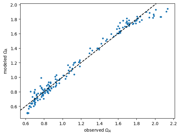
7.2. Assessing the model for bias#
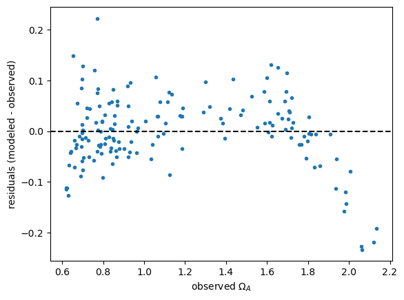
Plot model vs. observations. Note the systematic underestimate at high and low values of \(\Omega_A\). The residual plot shows this even more clearly.
plt.figure()
plt.plot(y,yhat,'.')
xl = plt.xlim()
yl = plt.ylim()
plt.plot(xl, xl, 'k--')
plt.xlim(xl)
plt.ylim(yl)
plt.xlabel('observed $\Omega_A$')
plt.ylabel('modeled $\Omega_A$');
Plot residuals vs. observations.
plt.figure()
plt.plot(y, yhat-y,'.')
xl = plt.xlim()
plt.plot(xl,[0,0],'k--')
plt.xlim(xl)
plt.xlabel('observed $\Omega_A$')
plt.ylabel('residuals (modeled - observed)');
Alternative approach using statsmodels#
Use statsmodels to get a complete summary of regression statistics. Note that the coefficients are the same as those obtained using Numpy above.
resultsm  = sm.OLS(y, X).fit()
print(resultsm.summary())
                            OLS Regression Results
==============================================================================
Dep. Variable:                 OmegaA   R-squared:                       0.976
Model:                            OLS   Adj. R-squared:                  0.975
Method:                 Least Squares   F-statistic:                     1230.
Date:                Mon, 13 Jan 2025   Prob (F-statistic):          1.44e-121
Time:                        11:28:22   Log-Likelihood:                 197.36
No. Observations:                 159   AIC:                            -382.7
Df Residuals:                     153   BIC:                            -364.3
Df Model:                           5
Covariance Type:            nonrobust
==============================================================================
                 coef    std err          t      P>|t|      [0.025      0.975]
------------------------------------------------------------------------------
const         -1.1903      2.013     -0.591      0.555      -5.167       2.787
x1            -0.0025      0.015     -0.169      0.866      -0.032       0.027
x2             0.0939      0.064      1.465      0.145      -0.033       0.220
x3             0.0003      0.000      2.105      0.037    2.07e-05       0.001
x4             0.0006      0.001      1.100      0.273      -0.000       0.002
x5            -0.0425      0.005     -7.968      0.000      -0.053      -0.032
==============================================================================
Omnibus:                       14.235   Durbin-Watson:                   0.755
Prob(Omnibus):                  0.001   Jarque-Bera (JB):               21.787
Skew:                           0.487   Prob(JB):                     1.86e-05
Kurtosis:                       4.530   Cond. No.                     7.67e+04
==============================================================================

Notes:
[1] Standard Errors assume that the covariance matrix of the errors is correctly specified.
[2] The condition number is large, 7.67e+04. This might indicate that there are
strong multicollinearity or other numerical problems.
resultsm.params
const   -1.190291
x1      -0.002516
x2       0.093875
x3       0.000337
x4       0.000562
x5      -0.042457
dtype: float64
c
array([-1.19029082e+00, -2.51555185e-03,  9.38753728e-02,  3.36570803e-04,
        5.61953385e-04, -4.24568174e-02])
Confronting multicollinearity#
In the output above, statsmodels gave a warning about a high condition number - this is an indicator of how much a small change to the matrix \(\textbf{X}\) will change the solution to the least squares problem \(\hat{c} = (\textbf{X}^T\textbf{X})^{-1}\textbf{X}^T\vec{y}\). It is a measure of the extent to which the columns in \(\textbf{X}\) are linearly independent and closely scaled in magnitude. The same condition number can be calculated using Numpy.
np.linalg.cond(X)
76723.09230168296
Multiple collinearity can also be assessed by looking at the correlation matrix (R) or calculating the variance inflation factor (VIF).
R = df07sub[['CTDTMP', 'CTDSAL', 'CTDPRS', 'CTDOXY', 'NITRAT']].corr()
R
| CTDTMP | CTDSAL | CTDPRS | CTDOXY | NITRAT | |
|---|---|---|---|---|---|
| CTDTMP | 1.000000 | -0.778421 | -0.772172 | 0.822573 | -0.863899 |
| CTDSAL | -0.778421 | 1.000000 | 0.770493 | -0.980860 | 0.979989 |
| CTDPRS | -0.772172 | 0.770493 | 1.000000 | -0.815279 | 0.786283 |
| CTDOXY | 0.822573 | -0.980860 | -0.815279 | 1.000000 | -0.985540 |
| NITRAT | -0.863899 | 0.979989 | 0.786283 | -0.985540 | 1.000000 |
VIF = 1/(1 - R**2)
VIF
| CTDTMP | CTDSAL | CTDPRS | CTDOXY | NITRAT | |
|---|---|---|---|---|---|
| CTDTMP | inf | 2.537683 | 2.476778 | 3.092395 | 3.942003 |
| CTDSAL | 2.537683 | inf | 2.460989 | 26.375274 | 25.238230 |
| CTDPRS | 2.476778 | 2.460989 | inf | 2.982225 | 2.619453 |
| CTDOXY | 3.092395 | 26.375274 | 2.982225 | inf | 34.830366 |
| NITRAT | 3.942003 | 25.238230 | 2.619453 | 34.830366 | inf |
Final model for aragonite saturation state#
Due to issues with bias and multiple collinearity, the following alternative model proposed by Juranek et al. (2009). It is simpler and contains an interaction term.
\( \hat{\Omega}_A = a_0 + a_1 \times (O - Oref) + a_2 \times (O - Oref) \times (T - Tref) \)
An important question is whether this model can predict aragonite saturation state in different years. This model can be tested using an independent data set from later cruises that cover the same region.