Cruise data analysis in Python

4. Cruise data analysis in Python#

4.1. WCOA 2013 data set#

To download the data used in this tutorial, use the following command in the Terminal (Mac) or Git Bash (Windows).

git clone https://github.com/mlmldata24/wcoa_cruise.git

The data comes from the West Coast Ocean Acidification (WCOA) cruise in 2013. The goal of this NOAA-supported research cruise is to collect data to help understand the effects of coastal upwelling on ocean acidification, and the impacts of ocean acidification on organisms and ecosystems. This video gives an idea of life aboard the ship and the type of science operations conducted.

In this part of the tutorial, we will go over the basics of working with dates in Pandas and Numpy, make some exploratory plots and start a regression analysis. The data exploration will be largely guided by student interest.

import numpy as np
import pandas as pd
from matplotlib import pyplot as plt
from scipy import stats

Introduction to Pandas dataframes#

We use Pandas to import the csv data file.

Here, there is an optional parse_dates argument. The numbers in double brackets [[8,9]] indicate which columns to interpret as dates.

filename = 'data/wcoa_cruise/WCOA2013_hy1.csv'
df = pd.read_csv(filename,header=31,na_values=-999,
                 parse_dates=[[8,9]])

/var/folders/z7/lmyk7sz94177j166ck0x63h80000gr/T/ipykernel_47173/3121988433.py:2: UserWarning: Could not infer format, so each element will be parsed individually, falling back to `dateutil`. To ensure parsing is consistent and as-expected, please specify a format.
  df = pd.read_csv(filename,header=31,na_values=-999,

df.head()

	DATE_TIME	EXPOCODE	SECT_ID	LEG	LINE	STNNBR	CASTNO	BTLNBR	BTLNBR_FLAG_W	LATITUDE	...	TCARBN	TCARBN_FLAG_W	ALKALI	ALKALI_FLAG_W	PH_TOT	PH_TOT_FLAG_W	PH_TMP	CO32	CO32__FLAG_W	CHLORA
0	2013-08-05 02:12:20	317W20130803	WCOA2013	1	2	11	1	1	2	48.2	...	2370.2	2	2369.0	2	7.294	2	25.0	NaN	9	NaN
1	2013-08-05 02:12:53	317W20130803	WCOA2013	1	2	11	1	2	2	48.2	...	NaN	9	NaN	9	7.295	2	25.0	NaN	9	NaN
2	2013-08-05 02:19:58	317W20130803	WCOA2013	1	2	11	1	3	2	48.2	...	2349.6	2	2343.7	2	7.282	2	25.0	43.521	3	NaN
3	2013-08-05 02:27:01	317W20130803	WCOA2013	1	2	11	1	4	2	48.2	...	2318.7	2	2311.9	2	7.287	2	25.0	45.641	2	NaN
4	2013-08-05 02:30:53	317W20130803	WCOA2013	1	2	11	1	5	2	48.2	...	2300.0	2	2299.7	2	7.308	2	25.0	47.741	2	NaN

5 rows × 42 columns

df.columns

Index(['DATE_TIME', 'EXPOCODE', 'SECT_ID', 'LEG', 'LINE', 'STNNBR', 'CASTNO',
       'BTLNBR', 'BTLNBR_FLAG_W', 'LATITUDE', 'LONGITUDE', 'DEPTH', 'CTDPRS',
       'CTDTMP', 'CTDSAL', 'CTDSAL_FLAG_W', 'CTDOXY', 'CTDOXY_FLAG_W',
       'SALNTY', 'SALNTY_FLAG_W', 'OXYGEN', 'OXYGEN_FLAG_W', 'SILCAT',
       'SILCAT_FLAG_W', 'NITRAT', 'NITRAT_FLAG_W', 'NITRIT', 'NITRIT_FLAG_W',
       'PHSPHT', 'PHSPHT_FLAG_W', 'AMMONI', 'AMMONI_FLAG_W', 'TCARBN',
       'TCARBN_FLAG_W', 'ALKALI', 'ALKALI_FLAG_W', 'PH_TOT', 'PH_TOT_FLAG_W',
       'PH_TMP', 'CO32', 'CO32__FLAG_W', 'CHLORA'],
      dtype='object')

Instead of strings, the dates are now in a special datetime64 format. This means that, instead of treating the dates in the same way as any other collection of characters, pandas and NumPy can understand how this variable represents time.

df['DATE_TIME'].head()

 2013-08-05 02:12:20
 2013-08-05 02:12:53
 2013-08-05 02:19:58
 2013-08-05 02:27:01
 2013-08-05 02:30:53
Name: DATE_TIME, dtype: datetime64[ns]

For example, subtracting datetime64 objects with pandas gives a Timedelta object, which is specifically used to represent differences between times. The first two samples in the cruise data are separated by 33 seconds (the time between firing of bottles).

df['DATE_TIME'][1]-df['DATE_TIME'][0]

Timedelta('0 days 00:00:33')

pd.unique(df['LATITUDE'])

array([48.2 , 48.3 , 48.37, 48.44, 48.5 , 48.53, 48.61, 48.66, 48.71,
       48.78, 48.81, 48.84, 47.97, 48.14, 47.96, 47.68, 47.13, 47.11,
       47.12, 47.34, 46.13, 46.17, 46.19, 46.25, 46.24, 46.12, 44.65,
       44.66, 44.2 , 41.99, 41.97, 41.96, 41.94, 41.9 , 40.25, 40.23,
       40.22, 40.21, 40.1 , 37.67, 37.94, 37.91, 37.87, 37.76, 37.75,
       36.8 , 36.78, 36.76, 36.73, 36.71, 36.69, 36.52, 36.7 ])

Exercise#

Create a list of unique station ID’s (“STNNBR”) found in the survey data. Call it stns. How many unique stations are there in the data?

Summary statistics#

A summary of the dataframe is given by the .describe() method.

df['CTDTMP'].describe()

count    969.000000
mean       8.993954
std        3.055917
min        1.738200
25%        7.292000
50%        8.328200
75%       10.752200
max       20.747400
Name: CTDTMP, dtype: float64

These summary statistics can also be accessed individually with similar syntax.

df['CTDTMP'].mean()

8.993954179566563

df['CTDTMP'].min()

1.7382

Alternate method using Numpy functions.

np.min(df['CTDTMP'])

1.7382

Mathematical operations#

Converting Celcius to Fahrenheit

df['CTDTMP_F'] = 9/5*df['CTDTMP'] + 32 

df['CTDTMP_F'].head()

  38.63894
  38.64236
  39.85916
  41.05328
  41.82404
Name: CTDTMP_F, dtype: float64

df['CTDTMP'].head()

  3.6883
  3.6902
  4.3662
  5.0296
  5.4578
Name: CTDTMP, dtype: float64

Plotting#

Plot latitude as a function of time.

plt.figure()
plt.plot(df['DATE_TIME'],df['LATITUDE'],'-o')
plt.xticks(rotation=15)

(array([15922., 15926., 15930., 15934., 15938., 15942., 15946.]),
 [Text(15922.0, 0, '2013-08-05'),
  Text(15926.0, 0, '2013-08-09'),
  Text(15930.0, 0, '2013-08-13'),
  Text(15934.0, 0, '2013-08-17'),
  Text(15938.0, 0, '2013-08-21'),
  Text(15942.0, 0, '2013-08-25'),
  Text(15946.0, 0, '2013-08-29')])

_images/5d24e115c85265b214f3bbc57b5087dcef85fd9476fc4b8604c07032e7cc0aa9.png

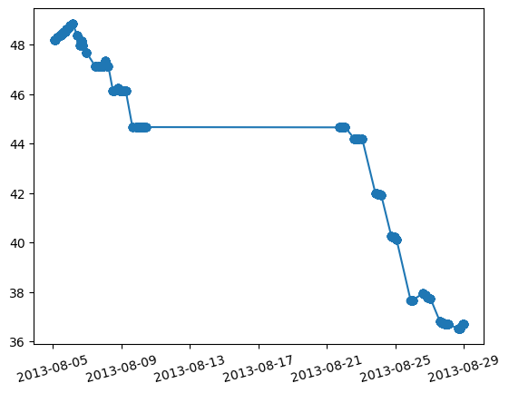
The pyplot library automatically understands datetime64 objects so it is easy to see how the ship moved between stations from north to south as weeks passed.

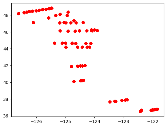
plt.figure()
plt.plot(df['LONGITUDE'], df['LATITUDE'], 'ro')

[<matplotlib.lines.Line2D at 0x143a27dd0>]

_images/6cd9df197153c91b85f8eb9f8e42e154432b6336f1f232e8e41a41142251c7f3.png

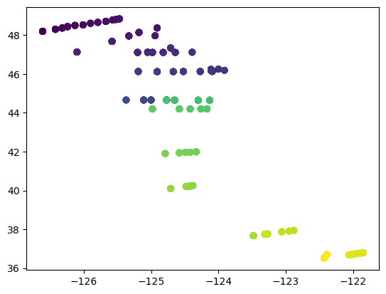
The scatter() function allows points to be colored according to the value of a variable. In the case of dates, later dates are shown as warmer colors.

plt.figure()
plt.scatter(df['LONGITUDE'],df['LATITUDE'],c=df['DATE_TIME'])

<matplotlib.collections.PathCollection at 0x143a3d6d0>

_images/cf06f33568c4e56159de0117470cdd9e216dabeaf1d8b6fc36150e2e6fdd9c21.png

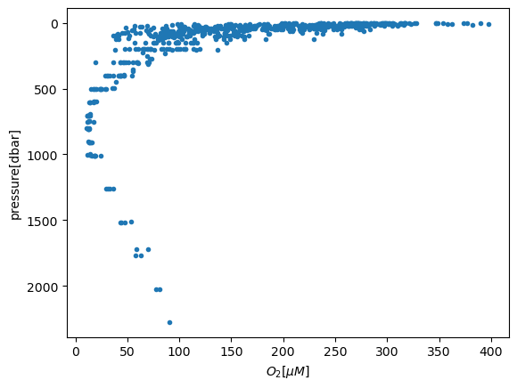
Note that the vertical coordinate is pressure (not depth, which indicates the bottom depth rather than the depth of the sample). To plot dissolved oxygen with depth:

plt.figure()
plt.plot(df['OXYGEN'],df['CTDPRS'],'.')
plt.gca().invert_yaxis()

plt.xlabel('$O_2 [\mu M]$')
plt.ylabel('pressure[dbar]')

Text(0, 0.5, 'pressure[dbar]')

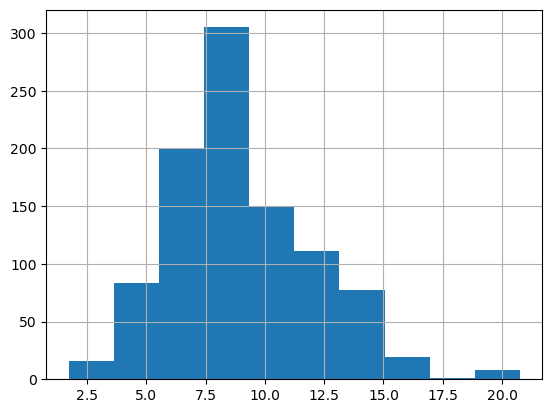
_images/ee868e9be2fe3b25692d10c47cb8925d7e22523a46671028e805251a3ffeeaa7.png

plt.figure()
df['CTDTMP'].hist()

<Axes: >

_images/1a1c29c010be44a9b99ef6c0d7d7b561367cfb35f65063ef82559ee6da16cd00.png

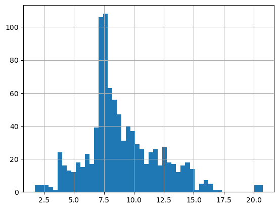
plt.figure()
df['CTDTMP'].hist(bins=50)

<Axes: >

_images/c505c5aa0349110a8854b46b5cb3f8ec6a4347274a1b1bc498a71640abe24385.png

df.keys()

Index(['DATE_TIME', 'EXPOCODE', 'SECT_ID', 'LEG', 'LINE', 'STNNBR', 'CASTNO',
       'BTLNBR', 'BTLNBR_FLAG_W', 'LATITUDE', 'LONGITUDE', 'DEPTH', 'CTDPRS',
       'CTDTMP', 'CTDSAL', 'CTDSAL_FLAG_W', 'CTDOXY', 'CTDOXY_FLAG_W',
       'SALNTY', 'SALNTY_FLAG_W', 'OXYGEN', 'OXYGEN_FLAG_W', 'SILCAT',
       'SILCAT_FLAG_W', 'NITRAT', 'NITRAT_FLAG_W', 'NITRIT', 'NITRIT_FLAG_W',
       'PHSPHT', 'PHSPHT_FLAG_W', 'AMMONI', 'AMMONI_FLAG_W', 'TCARBN',
       'TCARBN_FLAG_W', 'ALKALI', 'ALKALI_FLAG_W', 'PH_TOT', 'PH_TOT_FLAG_W',
       'PH_TMP', 'CO32', 'CO32__FLAG_W', 'CHLORA', 'CTDTMP_F'],
      dtype='object')

Exercises#

What scientific questions can be addressed with this data set?
What relationships might occur between different variables?
What differences might occur within the same variables, but at different locations or times?
Create exploratory plots (one PDF, one scatter plot)

4.2. Slicing and subsetting data#

df[0:3]

	DATE_TIME	EXPOCODE	SECT_ID	LEG	LINE	STNNBR	CASTNO	BTLNBR	BTLNBR_FLAG_W	LATITUDE	...	TCARBN_FLAG_W	ALKALI	ALKALI_FLAG_W	PH_TOT	PH_TOT_FLAG_W	PH_TMP	CO32	CO32__FLAG_W	CHLORA	CTDTMP_F
0	2013-08-05 02:12:20	317W20130803	WCOA2013	1	2	11	1	1	2	48.2	...	2	2369.0	2	7.294	2	25.0	NaN	9	NaN	38.63894
1	2013-08-05 02:12:53	317W20130803	WCOA2013	1	2	11	1	2	2	48.2	...	9	NaN	9	7.295	2	25.0	NaN	9	NaN	38.64236
2	2013-08-05 02:19:58	317W20130803	WCOA2013	1	2	11	1	3	2	48.2	...	2	2343.7	2	7.282	2	25.0	43.521	3	NaN	39.85916

3 rows × 43 columns

df.iloc[0:3]

	DATE_TIME	EXPOCODE	SECT_ID	LEG	LINE	STNNBR	CASTNO	BTLNBR	BTLNBR_FLAG_W	LATITUDE	...	TCARBN_FLAG_W	ALKALI	ALKALI_FLAG_W	PH_TOT	PH_TOT_FLAG_W	PH_TMP	CO32	CO32__FLAG_W	CHLORA	CTDTMP_F
0	2013-08-05 02:12:20	317W20130803	WCOA2013	1	2	11	1	1	2	48.2	...	2	2369.0	2	7.294	2	25.0	NaN	9	NaN	38.63894
1	2013-08-05 02:12:53	317W20130803	WCOA2013	1	2	11	1	2	2	48.2	...	9	NaN	9	7.295	2	25.0	NaN	9	NaN	38.64236
2	2013-08-05 02:19:58	317W20130803	WCOA2013	1	2	11	1	3	2	48.2	...	2	2343.7	2	7.282	2	25.0	43.521	3	NaN	39.85916

3 rows × 43 columns

df.loc[0:3]

	DATE_TIME	EXPOCODE	SECT_ID	LEG	LINE	STNNBR	CASTNO	BTLNBR	BTLNBR_FLAG_W	LATITUDE	...	TCARBN_FLAG_W	ALKALI	ALKALI_FLAG_W	PH_TOT	PH_TOT_FLAG_W	PH_TMP	CO32	CO32__FLAG_W	CHLORA	CTDTMP_F
0	2013-08-05 02:12:20	317W20130803	WCOA2013	1	2	11	1	1	2	48.2	...	2	2369.0	2	7.294	2	25.0	NaN	9	NaN	38.63894
1	2013-08-05 02:12:53	317W20130803	WCOA2013	1	2	11	1	2	2	48.2	...	9	NaN	9	7.295	2	25.0	NaN	9	NaN	38.64236
2	2013-08-05 02:19:58	317W20130803	WCOA2013	1	2	11	1	3	2	48.2	...	2	2343.7	2	7.282	2	25.0	43.521	3	NaN	39.85916
3	2013-08-05 02:27:01	317W20130803	WCOA2013	1	2	11	1	4	2	48.2	...	2	2311.9	2	7.287	2	25.0	45.641	2	NaN	41.05328

4 rows × 43 columns

df.loc[0:3,['CTDTMP','CTDPRS']]

	CTDTMP	CTDPRS
0	3.6883	999.5
1	3.6902	1000.8
2	4.3662	749.0
3	5.0296	503.9

Exercise#

What do you expect to happen when you execute:

df[0:1]
df[:4]
df[:-1]

What do you expect to happen when you call:

df.iloc[0:4, 1:4]
df.loc[0:4, 1:4]

How are the two commands different?

Adapted from: https://datacarpentry.org/python-ecology-lesson/03-index-slice-subset/index.html

Subsetting Data using Criteria#

df[df.LATITUDE > 40].head()

	DATE_TIME	EXPOCODE	SECT_ID	LEG	LINE	STNNBR	CASTNO	BTLNBR	BTLNBR_FLAG_W	LATITUDE	...	TCARBN_FLAG_W	ALKALI	ALKALI_FLAG_W	PH_TOT	PH_TOT_FLAG_W	PH_TMP	CO32	CO32__FLAG_W	CHLORA	CTDTMP_F
0	2013-08-05 02:12:20	317W20130803	WCOA2013	1	2	11	1	1	2	48.2	...	2	2369.0	2	7.294	2	25.0	NaN	9	NaN	38.63894
1	2013-08-05 02:12:53	317W20130803	WCOA2013	1	2	11	1	2	2	48.2	...	9	NaN	9	7.295	2	25.0	NaN	9	NaN	38.64236
2	2013-08-05 02:19:58	317W20130803	WCOA2013	1	2	11	1	3	2	48.2	...	2	2343.7	2	7.282	2	25.0	43.521	3	NaN	39.85916
3	2013-08-05 02:27:01	317W20130803	WCOA2013	1	2	11	1	4	2	48.2	...	2	2311.9	2	7.287	2	25.0	45.641	2	NaN	41.05328
4	2013-08-05 02:30:53	317W20130803	WCOA2013	1	2	11	1	5	2	48.2	...	2	2299.7	2	7.308	2	25.0	47.741	2	NaN	41.82404

5 rows × 43 columns

df[df.LATITUDE <= 40].head()

	DATE_TIME	EXPOCODE	SECT_ID	LEG	LINE	STNNBR	CASTNO	BTLNBR	BTLNBR_FLAG_W	LATITUDE	...	TCARBN_FLAG_W	ALKALI	ALKALI_FLAG_W	PH_TOT	PH_TOT_FLAG_W	PH_TMP	CO32	CO32__FLAG_W	CHLORA	CTDTMP_F
770	2013-08-25 21:23:35	32P020130821	WCOA2013	2	10	133	1	1	2	37.67	...	6	2430.4	6	7.493	2	25.0	73.346	2	NaN	35.12876
771	2013-08-25 21:32:13	32P020130821	WCOA2013	2	10	133	1	2	2	37.67	...	2	2427.6	2	7.467	2	25.0	69.812	2	NaN	35.30336
772	2013-08-25 21:40:44	32P020130821	WCOA2013	2	10	133	1	3	2	37.67	...	2	2424.3	2	7.442	2	25.0	65.502	2	NaN	35.55914
773	2013-08-25 21:49:45	32P020130821	WCOA2013	2	10	133	1	4	2	37.67	...	2	2413.7	2	7.400	2	25.0	60.170	2	NaN	36.10526
774	2013-08-25 21:57:55	32P020130821	WCOA2013	2	10	133	1	5	2	37.67	...	2	2401.4	2	7.374	2	25.0	57.739	2	NaN	36.92894

5 rows × 43 columns

dfsub = df[(df.CTDPRS <= 10) & (df.LATITUDE > 40)]

dfsub.head()

	DATE_TIME	EXPOCODE	SECT_ID	LEG	LINE	STNNBR	CASTNO	BTLNBR	BTLNBR_FLAG_W	LATITUDE	...	TCARBN_FLAG_W	ALKALI	ALKALI_FLAG_W	PH_TOT	PH_TOT_FLAG_W	PH_TMP	CO32	CO32__FLAG_W	CHLORA	CTDTMP_F
18	2013-08-05 03:00:52	317W20130803	WCOA2013	1	2	11	1	19	4	48.20	...	9	NaN	9	NaN	9	NaN	NaN	9	NaN	56.54660
19	2013-08-05 03:01:10	317W20130803	WCOA2013	1	2	11	1	20	2	48.20	...	2	2189.1	6	7.983	3	25.0	155.043	2	NaN	56.54570
38	2013-08-05 06:37:22	317W20130803	WCOA2013	1	2	12	1	19	2	48.30	...	9	2180.0	6	7.980	3	25.0	152.868	2	NaN	57.72218
39	2013-08-05 06:37:42	317W20130803	WCOA2013	1	2	12	1	20	2	48.30	...	2	NaN	9	7.981	2	25.0	NaN	5	NaN	57.72290
58	2013-08-05 10:41:19	317W20130803	WCOA2013	1	2	13	1	19	2	48.37	...	2	2178.7	2	7.931	2	25.0	142.629	2	NaN	55.69844

5 rows × 43 columns

Exercises#

Select a subset of rows in the df DataFrame that contains data from a pressure range between 500 and 1000 dbar. How many rows did you end up with? What did your neighbor get?
You can use the isin command in Python to query a DataFrame based upon a list of values as follows:

df[df['STNNBR'].isin([listGoesHere])]

Use the isin function to find all samples from station numbers 11 and 12.

Exercises#

pH values are contained in the df['PH_TOT'] DataArray

Quality control flags for pH are contained in the df['PH_TOT_FLAG_W'] DataArray.

World Ocean Circulation Experiment (WOCE) quality control flags are used:

2 = good value
3 = questionable value
4 = bad value
5 = value not reported
6 = mean of replicate measurements
9 = sample not drawn.

1. Create a new DataFrame called dfsub1 that includes only data where pressure is less than 10 dbar and the latitude is farher north than \(40^{\circ} \text{N}\).

Create a new DataFrame called dfsub2 that excludes all bad, questionable and missing pH and CTD oxygen values. Plot oxygen vs. pH.

Fit a linear model in Python#

plt.plot(df['CTDOXY'],df['PH_TOT'],'.')
plt.xlabel('dissolved oxygen [$\mu$mol/kg]')
plt.ylabel('pH$_{Tot}$')

Text(0, 0.5, 'pH$_{Tot}$')

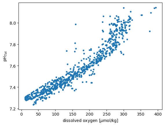
_images/8d5982d79f2633017fdaecd2ed6d176cef8c52d8783546a82beda94269cbfca7.png

result = stats.linregress(dfsub2['CTDOXY'],dfsub2['PH_TOT'])

result

LinregressResult(slope=0.002305076546103237, intercept=7.202036145940105, rvalue=0.9510631019969654, pvalue=0.0, stderr=2.7737424376777354e-05, intercept_stderr=0.004977802641597415)

Exercise#

Plot the linear model with the data.

Cruise data analysis in Python

Contents

4. Cruise data analysis in Python#

4.1. WCOA 2013 data set#

Introduction to Pandas dataframes#

Exercise#

Summary statistics#

Mathematical operations#

Plotting#

Exercises#

4.2. Slicing and subsetting data#

Exercise#

Subsetting Data using Criteria#

Exercises#

Exercises#

Fit a linear model in Python#

Exercise#